Introduction
Interestingly, a significant portion of machine learning revolves around optimization and the reason this is is because of the task of a model needing to learn to better improve their predictions for the target outputs—in machine-learning adjacent roles, you might see that that they want someone with experience with specifically convex optimization. We’ll take this challenge of teaching a model to learn with a mathematical spirit, and this journal entry aims to explain this concisely but also, hopefully, clearly.
When measuring how well our model’s prediction is matching the target outputs with a loss function, the goal of learning is to find the model parameters (e.g., weights, biases, etc) which minimize the loss function. In practice, one of the most common strategies for optimization is the technique of Gradient Descent—the term “gradient” making some allusions to analysis.
Suppose we have a dataset $D_N = \{(x_i, y_i ) \}_{i=1}^N$ where each $x_i \in \mathbf R^d$ is an input/feature vector and $y_i$ is the corresponding target output (e.g. $y_i$ could be real for regression, or a class label for classification). We prepose a model function $f_\theta \colon \mathbf R^d \to \mathbf R^k$ governed by parameters $\theta \in \mathbf R^m$—this model function could be a linear model such as linear regression, a neural network (NN). Now define a loss function \(\mathcal{L}\bigl(f_\theta(x), y\bigr)\) which measures the discrepancy between the prediction, $f_\theta(x)$, and the true label, $y$. For classification, a common choice is the cross-entropy loss; for regression, we typically use MSE: \[\mathcal{L}\bigl(f_\theta(x), y\bigr) = \frac{1}{N} \sum_{i=1}^N \bigl(f_\theta(x_i) - y_i\bigr)^2, \]and for a linear model we have $f_\theta(x) = w^T x + b$ and $\theta = \{w, b \}$ where $w$ is a vector of coefficients and $b$ is the bias. In general, the overall cost (or objective) function is typically expressed as an average loss over all training samples:
\[C(\theta) \;=\; \frac{1}{N} \sum_{i=1}^N \mathcal{L}\bigl(f_\theta(x_i), y_i \bigr), \] and our aim is to find \[ \theta^* \;=\; \underset{\theta}{\operatorname{argmin}}\; C(\theta). \]
Into gradient descent
The gradient descent technique is an iterative process to find (local) minima of a real valued function, and in our narrow case we want to minimize $C(\theta)$. Recall that the gradient of $C(\theta)$ is just $\nabla_\theta C(\theta) = \left ( \frac{\partial C}{\partial \theta_1 }, \frac{\partial C}{\partial \theta_2}, \ldots, \frac{\partial C}{\partial \theta_m} \right ).$ Importantly, this gradient vector points in the direction of steepest increase of C, which is an essential property in our gradient descent process: gradient descent states that if you want to move $\theta$ in a direction that reduces $C(\theta)$, you should step against (i.e., in the negative direction of) the gradient. So, with this in mind, we setup the updating rule $\theta_{\text{new}} = \theta_{\text{old}} - \eta \nabla_\theta C(\theta) $ where $\eta > 0$ is the learning rate (typically a small scaler). We perform this updating (often called the “gradient descent step”) many times until we hopefully) converge to a minimum:
\[ \theta^{(t+1)} \;=\;\theta^{(t)} \;-\; \eta \,\nabla_\theta C\bigl(\theta^{(t)}\bigr). \]
In an ideal world, to check that we have a minimum on our hands, we would want to check that we have a stationary point, $\nabla_\theta C(\theta) = 0 $ but we would also need to check that the Hessian matrix of $C(\theta)$, $\nabla^2_\theta C(\theta)$, is positive semidefinite—this would indicate a local minimum. However, machine learning gives rise to computationally difficult world whereby this isn’t usually the method/heuristic we use to verify that we have a minimum. In practical machine learning, especially high-dimensional (lots and lots of parameters, i.e. $\theta \in \mathbf R^N$ where $N$ is big), non-convex landscapes, we instead rely on stopping criteria—useful heuristics which inform us that our iterative procedure is “good enough” or unlikely to produce something substantially better. Some common stopping criteria are:
Stop when $ \|\nabla_\theta C(\theta)\|$ drops below a small threshold (e.g. $10^{-5}$). The reasoning behind this is that a very small gradient suggests we are near a stationary point (although it could be a minimum, maximum, or saddle).
Stop when \(\bigl|C(\theta^{(t+1)}) - C(\theta^{(t)})\bigr|\) becomes negligibly small. If the objective is no longer decreasing significantly, further iterations may yield minimal improvement.
Stop when $\|\theta^{(t+1)} - \theta^{(t)}\|$ is below a threshold. If the parameters hardly change with each step, it indicates that the algorithm is converging or stuck.
In practice, due to time or resource limits, we might set a maximum number of epochs or a time budget.
What’s also important to note here is that you’re strategize/technique for gradient descent will vary if whether or not you’re in a convex vs. non-convex environment. In the non-convex world, functions, like those that arise in deep neural networks, have many stationary points, including a local minima and saddle points. So, a small gradient indicates that you’ve found a stationary point, but this is not guaranteed to be a global or even local minimum. Formally proving you’ve reached the global minimum is usually intractable for non-convex problems. But these standard convergence heuristics are sufficient in most machine learning contexts to declare that “training is done.”
Example. Implementing gradient descent for single variable linear regression:

Convex vs. non-convex
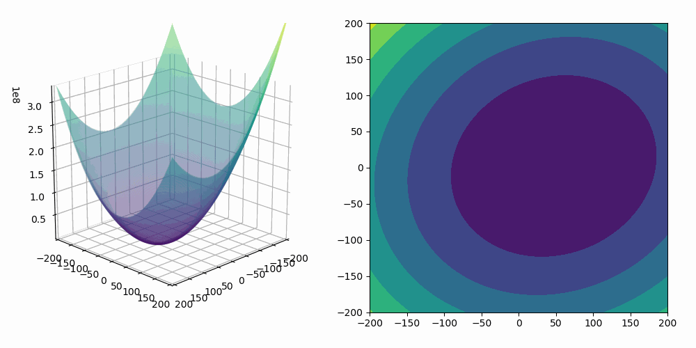
In optimization theory, the convex vs. non-convex distinction is crucial—fundamentally altering how easy or hard it is to find (as well as verify) a global minimum. To further dig into why this is crucial, recall that a function $f \colon \mathbf R^n \to \mathbf R$ is convex if for all $x, y \in \mathbf R^n$ and all $\lambda \in [0,1]$, $f(\lambda x + (1-\lambda)y) \leq \lambda f(x) + (1-\lambda) f(y)$ holds. This property is realized, geometrically, as any line segment between two points on the graph of $f$ lies above or on the graph, e.g. Also, convex functions have the property that any local minimum is automatically a global minimum.
Lemma. If $f$ is convex, then a local minimum is in fact a global minimum.
Proof. Let \( f \) be a convex function, and let \( x^* \) be a local minimum. By definition of a local minimum, there exists a neighborhood \( N \) around \( x^* \) such that \( f(x^*) \leq f(x) \) for all \( x \in N \). Suppose, for contradiction, that \( x^* \) is not a global minimum. Then there exists some \( y \) such that \( f(y) < f(x^*) \). By convexity of \( f \), for any \( \lambda \in (0, 1) \): \[ f(\lambda x^* + (1-\lambda)y) \leq \lambda f(x^*) + (1-\lambda)f(y) < \lambda f(x^*) + (1-\lambda)f(x^*) = f(x^*).\] For \( \lambda \) sufficiently close to 1, \( \lambda x^* + (1-\lambda)y \) lies in the neighborhood \( N \), contradicting the fact that \( x^* \) is a local minimum. Therefore, \( x^* \) must be a global minimum. \(\square\)

